Binding Free Energy Tutorial
General BFE background
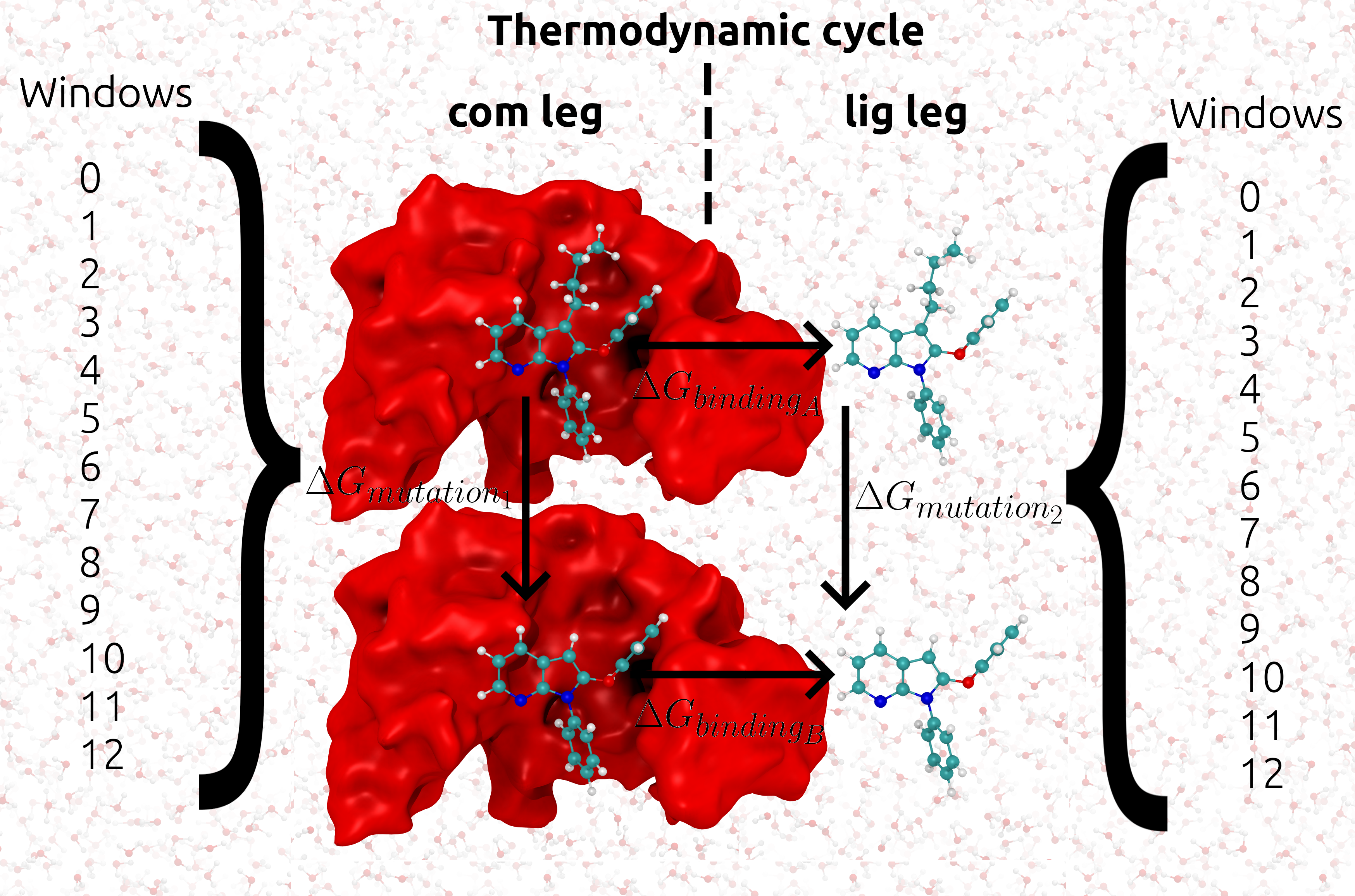
The discussion in the Tutorial section outlines performing one alchemical simulation with TIES_MD
for a binding free energy calculation we need two alchemical simulations. We call these two simulations
the complex and ligand simulations shortened to com and lig respectively. The lig simulation transforms one ligand A
into another B in water the com simulation does the same but now inside the protein. The com and lig simulations
give us \({Δ G_{mutation1}}\) and \({Δ G_{mutation2}}\) respectively the difference of these values is equal
to the binding free energy \({ΔΔ G}\). This idea of complex and ligand simulations relating to the difference
in binding free energy is shown in the following figure:
More details of these methods can be found in the publications of Cournia et al..
When we discuss the running of X replica simulations this whole thermodynamic cycle is run X times. To run the com and
lig simulations these must be setup by hand or by using TIES20. Setting up the lig and com simulations follows the same
principles as discussed in the Tutorial section. Some additional ideas however are that a constraints file is normally
used for the com simulation, this is included to avoid rapid changes of the protein crystal structure conformation early
in the simulation, caused by close atom contacts. Also the com simulation will contain more atoms and so be more expensive
computationally.
Setup
To set up these calculation we recommend the use of TIES20. This is a program designed to both build and parameterize
hybrid ligands but also setup binding free energy calculations for the TIES protocol that can be run with TIES_MD.
TIES20 can be used in browser. Alternatively one can use the TIES20 API to set up
simulations. In order to use the API TIES20 must be installed locally please see the TIES20 git.
for how to do this. With TIES20 installed you can use the API as follows to build inputs:
#ties20 imports
from ties import Pair, Config, Ligand, Protein

#Setting for system building
config = Config()
config.ligand_ff_name = 'gaff2'
config.ligand_net_charge = 0
config.md_engine = 'openmm'

#prep ligandA
ligandA = Ligand('ligandA.mol2', config=config)
ligandA.antechamber_prepare_mol2()

#prep ligandB
ligandB = Ligand('ligandB.mol2', config=config)
ligandB.antechamber_prepare_mol2()

#make ligandA and ligandB into a pair
pair = Pair(ligandA, ligandB, ligand_net_charge=config.ligand_net_charge, config=config)

#ensure the names of all atoms are different (needed for hybridizing)
pair.make_atom_names_unique()

#turn the pair into a hybrid
hybrid = pair.superimpose()

#Since no protein is declared this will build lig simulation
hybrid.prepare_inputs()

#now declare protein
config.protein = 'receptor.pdb'
config.protein_ff = 'leaprc.protein.ff14SB'
protein = Protein(config)

#re-prepare simulation input, now protein is declared and passed as argument com simulation is built
hybrid.prepare_inputs(protein=protein)
This will build all the input needed to run a BFE calculation for the \({ΔΔ G}\) between ligandA and ligandB. However, in order to run at this point the user must execute their own HPC submission scripts or run via the command line on a cluster. We can however build own submission scripts and or change any of the simulation setting as detailed in the next section.
Running
At this point we have prepped a simulation of one thermodynamic cycle with two legs named lig and com. TIES20 will
set these legs up in the directories ties/ties-ligandA-ligandB/(lig/com) and these map to the
system/ligand/thermodynamic_leg/ directory structure that was discussed in the Tutorial section.
In ties/ties-ligandA-ligandB/(lig/com) there will be the build directory and TIES.cfg files as also seen in
the Tutorial. The automatic settings in TIES.cfg will be good for a default simulation but in general we may wish to
change these quickly and or write submission scripts for these simulations. To do this we can use the TIES_MD API as
follows:
#tiesMD imports
from TIES_MD import TIES
import os

#iterate over both legs of BFE calculation
for thermo_leg in ['com', 'lig']:
    #point to the simulation directory
    ties_dir = os.path.join(os.getcwd(), 'ties', 'ties-ligandA-ligandB', thermo_leg)

    #read the default TIES.cfg to initialize
    md = TIES(ties_dir)

    #change some settings in TIES.cfg
    md.split_run = 1
    md.total_reps = 6

    #inspect all the options we can configure and change
    md.get_options()

    #change the header of generated submission scripts
    md.sub_header = """#Example script for Summit OpenMM
#BSUB -P CHM155_001
#BSUB -W 120
#BSUB -nnodes 13
#BSUB -alloc_flags "gpudefault smt1"
#BSUB -J LIGPAIR
#BSUB -o oLIGPAIR.%J
#BSUB -e eLIGPAIR.%J"""

    #Setting HPC specific elements of run line (example here is Summit)
    md.pre_run_line = 'jsrun --smpiargs="off" -n 1 -a 1 -c 1 -g 1 -b packed:1 '

    #Setting ties_md part of run line
    md.run_line = 'ties_md --config_file=$ties_dir/TIES.cfg --windows_mask=$lambda,$(expr $lambda + 1) --node_id=$i'

    #setup the new simulation with changed options (also writes submission script)
    md.setup()
This changes the TIES.cfg options split_run to 1 (True) and total_reps to 6. To see all configurable options the user
can run md.get_options() as shown above. To generate a general submission script we are modifying the
sub_header, pre_run_line and run_line internal options and these set what TIES_MD writes into the
submission script, for more details see API. These scripts can be summited to the HPC scheduler, once they
finish the last step to get a \({ΔΔ G}\) is analysis.
BFE Analysis
Once the simulations are finished the analysis can be performed as discussed in the Tutorial section. If we are in
the ties/ties-ligandA-ligandB/(lig/com) directory run:
cd ../../..
ties_ana --run_type=setup
Then modify the analysis.cfg file such the legs option is now to legs = lig, com (the two legs of our cycle). Note,
configured like this the \({ΔΔ G}\) is computed as the \({Δ G}\) of the ligand simulation minus the \({Δ G}\)
of the complex simulation, take care this gives you the same \({ΔΔ G}\) as you want to compare to in experiment
and it depends on which ligand is ligandA/B in the cycle. Running the following command will once again give
a results.dat file as output:
ties_ana
results.dat file file will have the same format as in the Tutorial section but it now
contains the \({ΔΔ G}\) of each transformation and the associated standard error of the mean (SEM). The print out on
the terminal will detail the individual \({Δ G}\) results for each thermodynamic leg.